Convolutional Neural Networks Cheatsheet

Learn more about convolutional neural networks from these resources from Stanford University to assist you on your journey through our Kambria Code Challenge: Quiz 02. Top-scoring developers will have an opportunity to have their resume and profile sent to Kambria’s corporate partners for career opportunities, so be sure to study hard, and you'll have the opportunity to take home some exceptional prizes!

Overview - Convolutional Neural Networks

Architecture of a traditional CNN ― Convolutional neural networks, also known as CNNs, are a specific type of neural network generally composed of the following layers:

The convolution layer and the pooling layer can be fine-tuned with respect to hyperparameters that are described in the next sections.

Types of layers

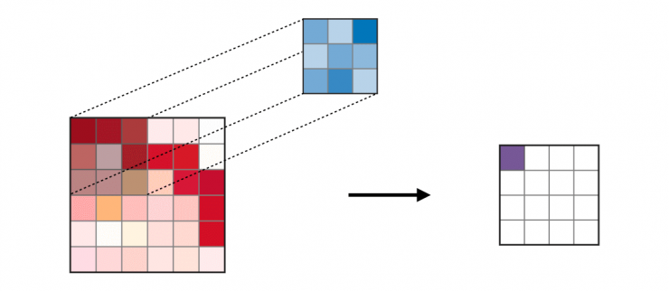
Convolution layer (CONV) ― The convolution layer (CONV) uses filters that perform convolution operations as it is scanning the input $I$ with respect to its dimensions. Its hyperparameters include the filter size $F$ and stride $S$ . The resulting output $O$ is called a feature map or activation map.

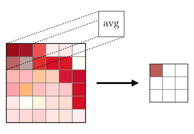
Remark: the convolution step can be generalized to the 1D and 3D cases as well.

Pooling (POOL) ― The pooling layer (POOL) is a downsampling operation, typically applied after a convolution layer, which does some spatial invariance. In particular, max and average pooling are special kinds of pooling where the maximum and average value is taken, respectively.

Type	Max pooling	Average pooling
Purpose	Each pooling operation selects the maximum value of the current view	Each pooling operation averages the values of the current view
Illustration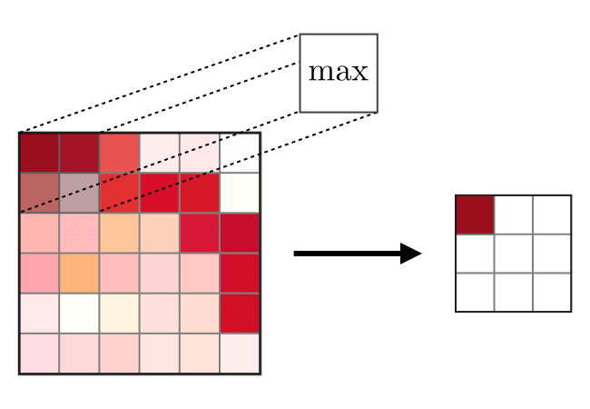
Comments	• Preserves detected features • Most commonly used	• Downsamples feature map • Used in LeNet

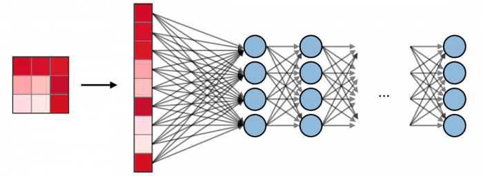
Fully Connected (FC) ― The fully connected layer (FC) operates on a flattened input where each input is connected to all neurons. If present, FC layers are usually found towards the end of CNN architectures and can be used to optimize objectives such as class scores.

Filter hyperparameters

The convolution layer contains filters for which it is important to know the meaning behind its hyperparameters.

Dimensions of a filter ― A filter of size $F\times F$ applied to an input containing $C$ channels is a $F\times F\times C$ volume that performs convolutions on an input of size $I\times I\times C$ and produces an output feature map (also called activation map) of size $O\times O\times 1$ .

Remark: the application of $K$ filters of size $F\times F$ results in an output feature map of size $O\times O\times K$ .

Stride ― For a convolutional or a pooling operation, the stride $S$ denotes the number of pixels by which the window moves after each operation.

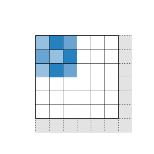
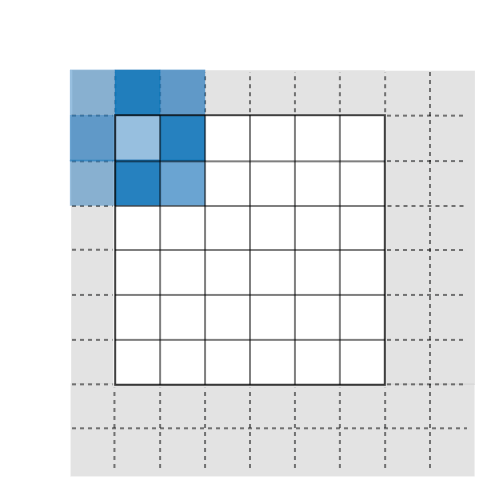
Zero-padding ― Zero-padding denotes the process of adding $P$ zeroes to each side of the boundaries of the input. This value can either be manually specified or automatically set through one of the three modes detailed below:

Mode	Valid	Same	Full
Value	$P=0$	$P_\text{start} = \Bigl\lfloor\frac{S \lceil\frac{I}{S}\rceil - I + F - S}{2}\Bigr\rfloor$ $P_\text{end} = \Bigl\lceil\frac{S \lceil\frac{I}{S}\rceil - I + F - S}{2}\Bigr\rceil$	$P_\text{start}\in[\![0,F-1]\!]$ $P_\text{end} = F-1$
Illustration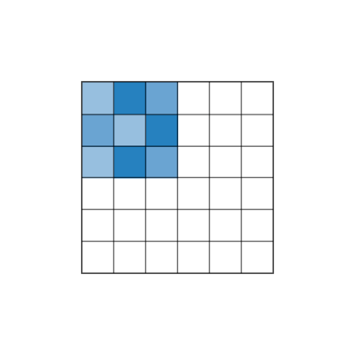
Purpose	• No padding • Drops last convolution if dimensions do not match	• Padding such that feature map size has size $\Bigl\lceil\frac{I}{S}\Bigr\rceil$ • Output size is mathematically convenient • Also called 'half' padding	• Maximum padding such that end convolutions are applied on the limits of the input • Filter 'sees' the input end-to-end

Tuning hyperparameters

Parameter compatibility in convolution layer ― By noting $I$ the length of the input volume size, $F$ the length of the filter, $P$ the amount of zero padding, $S$ the stride, then the output size $O$ of the feature map along that dimension is given by:

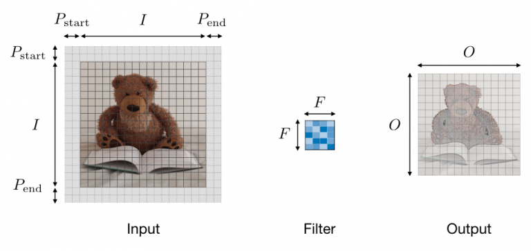
$\boxed{O=\frac{I-F+P_\text{start} + P_\text{end}}{S}+1}$

Remark: often times, $P_\text{start} = P_\text{end} \triangleq P$ , in which case we can replace $P_\text{start} + P_\text{end}$ by $2P$ in the formula above.

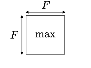
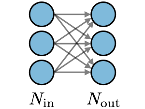
Understanding the complexity of the model ― In order to assess the complexity of a model, it is often useful to determine the number of parameters that its architecture will have. In a given layer of a convolutional neural network, it is done as follows:

CONV	POOL	FC
Illustration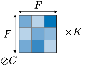
Input size	$I \times I \times C$	$I \times I \times C$	$N_{\text{in}}$
Output size	$O \times O \times K$	$O \times O \times C$	$N_{\text{out}}$
Number of parameters	$(F \times F \times C + 1) \cdot K$	0	$(N_{\text{in}} + 1 ) \times N_{\text{out}}$
Remarks	• One bias parameter per filter • In most cases, $S < F$ • A common choice for $K$ is $2C$	• Pooling operation done channel-wise • In most cases, $S=F$	• Input is flattened • One bias parameter per neuron • The number of FC neurons is free of structural constraints

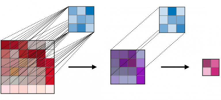
Receptive field ― The receptive field at layer $k$ is the area denoted $R_k \times R_k$ of the input that each pixel of the $k$ -th activation map can 'see'. By calling $F_j$ the filter size of layer $j$ and $S_i$ the stride value of layer $i$ and with the convention $S_0=1$ , the receptive field at layer $k$ can be computed with the formula:

$\boxed{R_k = 1 + \sum_{j=1}^{k} (F_j - 1) \prod_{i=0}^{j-1} S_i}$

In the example below, we have $F_1 = F_2 = 3$ and $S_1 = S_2 = 1$ , which gives $R_2 = 1 + 2\cdot 1 + 2\cdot 1 = 5$ .

Commonly used activation functions

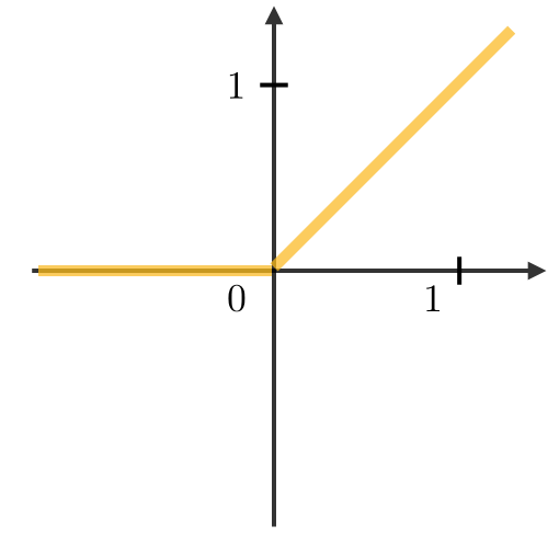
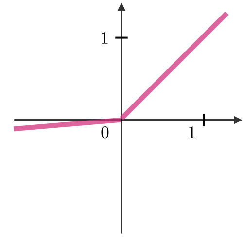
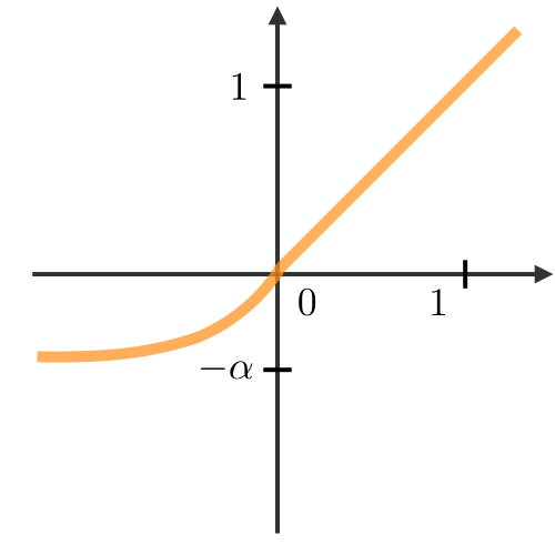
Rectified Linear Unit ― The rectified linear unit layer (ReLU) is an activation function $g$ that is used on all elements of the volume. It aims at introducing non-linearities to the network. Its variants are summarized in the table below:

ReLU	Leaky ReLU	ELU
$g(z)=\max(0,z)$	$g(z)=\max(\epsilon z,z)$ with $\epsilon\ll1$	$g(z)=\max(\alpha(e^z-1),z)$ with $\alpha\ll1$

• Non-linearity complexities biologically interpretable	• Addresses dying ReLU issue for negative values	• Differentiable everywhere

Softmax ― The softmax step can be seen as a generalized logistic function that takes as input a vector of scores $x\in\mathbb{R}^n$ and outputs a vector of output probability $p\in\mathbb{R}^n$ through a softmax function at the end of the architecture. It is defined as follows:

$\boxed{p=\begin{pmatrix}p_1\\\vdots\\p_n\end{pmatrix}}\quad\textrm{where}\quad\boxed{p_i=\frac{e^{x_i}}{\displaystyle\sum_{j=1}^ne^{x_j}}}$

Object detection

Types of models ― There are 3 main types of object recognition algorithms for which the nature of what is predicted is different. They are described in the table below:

Image classification	Classification w. localization	Detection

• Classifies a picture • Predicts the probability of the object	• Detects an object in a picture • Predicts the probability of the object and where it is located	• Detects up to several objects in a picture • Predicts probabilities of objects and where they are located
Traditional CNN	Simplified YOLO, R-CNN	YOLO, R-CNN

Detection ― In the context of object detection, different methods are used depending on whether we just want to locate the object or detect a more complex shape in the image. The two main ones are summed up in the table below:

Bounding box detection	Landmark detection
• Detects the part of the image where the object is located	• Detects a shape or characteristics of an object (e.g. eyes) • More granular

Box of center $(b_x,b_y)$ , height $b_h$ and width $b_w$	Reference points $(l_{1x},l_{1y}),...,(l_{nx},l_{ny})$

Intersection over Union ― Intersection over Union, also known as $\textrm{IoU}$ , is a function that quantifies how correctly positioned a predicted bounding box $B_p$ is over the actual bounding box $B_a$ . It is defined as:

$\boxed{\textrm{IoU}(B_p,B_a)=\frac{B_p\cap B_a}{B_p\cup B_a}}$

Remark: we always have $\textrm{IoU}\in[0,1]$ . By convention, a predicted bounding box $B_p$ is considered as being reasonably good if $\textrm{IoU}(B_p,B_a)\geqslant0.5$ .

Anchor boxes ― Anchor boxing is a technique used to predict overlapping bounding boxes. In practice, the network is allowed to predict more than one box simultaneously, where each box prediction is constrained to have a given set of geometrical properties. For instance, the first prediction can potentially be a rectangular box of a given form, while the second will be another rectangular box of a different geometrical form.

Non-max suppression ― The non-max suppression technique aims at removing duplicate overlapping bounding boxes of the same object by selecting the most representative ones. After having removed all boxes having a probability prediction lower than 0.6, the following steps are repeated while there are boxes remaining:

For a given class,
• Step 1: Pick the box with the largest prediction probability.
• Step 2: Discard any box having an $\textrm{IoU}\geqslant0.5$ with the previous box.

YOLO ― You Only Look Once (YOLO) is an object detection algorithm that performs the following steps:

• Step 1: Divide the input image into a $G\times G$ grid.
• Step 2: For each grid cell, run a CNN that predicts $y$ of the following form:

$\boxed{y=\big[\underbrace{p_c,b_x,b_y,b_h,b_w,c_1,c_2,...,c_p}_{\textrm{repeated }k\textrm{ times}},...\big]^T\in\mathbb{R}^{G\times G\times k\times(5+p)}}$

where $p_c$ is the probability of detecting an object, $b_x,b_y,b_h,b_w$ are the properties of the detected bouding box, $c_1,...,c_p$ is a one-hot representation of which of the $p$ classes were detected, and $k$ is the number of anchor boxes.
• Step 3: Run the non-max suppression algorithm to remove any potential duplicate overlapping bounding boxes.

Remark: when $p_c=0$ , then the network does not detect any object. In that case, the corresponding predictions $b_x, ..., c_p$ have to be ignored.

R-CNN ― Region with Convolutional Neural Networks (R-CNN) is an object detection algorithm that first segments the image to find potential relevant bounding boxes and then run the detection algorithm to find most probable objects in those bounding boxes.

Region with Convolutional Neural Networks (R-CNN) is an object detection algorithm that first segments the image to find potential relevant bounding boxes and then run the detection algorithm to find most probable objects in those bounding boxes.

Remark: although the original algorithm is computationally expensive and slow, newer architectures enabled the algorithm to run faster, such as Fast R-CNN and Faster R-CNN.

Face verification and recognition

Types of models ― Two main types of model are summed up in the table below:

Face verification	Face recognition
• Is this the correct person? • One-to-one lookup	• Is this one of the $K$ persons in the database? • One-to-many lookup

One Shot Learning ― One Shot Learning is a face verification algorithm that uses a limited training set to learn a similarity function that quantifies how different two given images are. The similarity function applied to two images is often noted $d(\textrm{image 1}, \textrm{image 2}).$ $d (image 1, image 2) .$

Siamese Network ― Siamese Networks aim at learning how to encode images to then quantify how different two images are. For a given input image $x^{(i)}$ , the encoded output is often noted as $f(x^{(i)})$ .

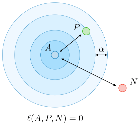
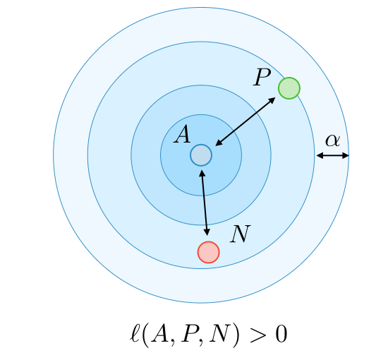
Triplet loss ― The triplet loss $\ell$ is a loss function computed on the embedding representation of a triplet of images $A$ (anchor), $P$ (positive) and $N$ (negative). The anchor and the positive example belong to a same class, while the negative example to another one. By calling $\alpha\in\mathbb{R}^+$ the margin parameter, this loss is defined as follows:

$\boxed{\ell(A,P,N)=\max\left(d(A,P)-d(A,N)+\alpha,0\right)}$

The triplet loss ℓℓ is a loss function computed on the embedding representation of a triplet of images AA (anchor), PP (positive) and NN (negative).

Neural style transfer

Motivation ― The goal of neural style transfer is to generate an image $G$ based on a given content $C$ and a given style $S$ .

Activation ― In a given layer $l$ , the activation is noted $a^{[l]}$ and is of dimensions $n_H\times n_w\times n_c$

Content cost function ― The content cost function $J_{\textrm{content}}(C,G)$ is used to determine how the generated image $G$ differs from the original content image $C$ . It is defined as follows:

$\boxed{J_{\textrm{content}}(C,G)=\frac{1}{2}||a^{[l](C)}-a^{[l](G)}||^2}$

Style matrix ― The style matrix $G^{[l]}$ of a given layer $l$ is a Gram matrix where each of its elements $G_{kk'}^{[l]}$ quantifies how correlated the channels $k$ and $k'$ are. It is defined with respect to activations $a^{[l]}$ as follows:

$\boxed{G_{kk'}^{[l]}=\sum_{i=1}^{n_H^{[l]}}\sum_{j=1}^{n_w^{[l]}}a_{ijk}^{[l]}a_{ijk'}^{[l]}}$

Remark: the style matrix for the style image and the generated image are noted $G^{[l](S)}$ and $G^{[l](G)}$ respectively.

Style cost function ― The style cost function $J_{\textrm{style}}(S,G)$ is used to determine how the generated image $G$ differs from the style $S$ . It is defined as follows:

$\boxed{J_{\textrm{style}}^{[l]}(S,G)=\frac{1}{(2n_Hn_wn_c)^2}||G^{[l](S)}-G^{[l](G)}||_F^2=\frac{1}{(2n_Hn_wn_c)^2}\sum_{k,k'=1}^{n_c}\Big(G_{kk'}^{[l](S)}-G_{kk'}^{[l](G)}\Big)^2}$

Overall cost function ― The overall cost function is defined as being a combination of the content and style cost functions, weighted by parameters $\alpha,\beta$ as follows:

$\boxed{J(G)=\alpha J_{\textrm{content}}(C,G)+\beta J_{\textrm{style}}(S,G)}$

Remark: a higher value of $\alpha$ will make the model care more about the content while a higher value of $\beta$ will make it care more about the style.

Architectures using computational tricks

Generative Adversarial Network ― Generative adversarial networks, also known as GANs, are composed of a generative and a discriminative model, where the generative model aims at generating the most truthful output that will be fed into the discriminative which aims at differentiating the generated and true image.

Remark: use cases using variants of GANs include text to image, music generation and synthesis.

ResNet ― The Residual Network architecture (also called ResNet) uses residual blocks with a high number of layers meant to decrease the training error. The residual block has the following characterizing equation:

$\boxed{a^{[l+2]}=g(a^{[l]}+z^{[l+2]})}$ Inception Network ― This architecture uses inception modules and aims at giving a try at different convolutions in order to increase its performance through features diversification. In particular, it uses the $1\times 1$ convolution trick to limit the computational burden.

To learn more, or to join the Kambria Code Challenge: Quiz 02, be sure to read the official announcement, including information on how you can win additional prizes by signing up early (restrictions apply). For more info, please visit: https://bit.ly/KambriaQuiz02Announcement. Thank you and good luck!

Source: Stanford